Run Acres Per Hour Calculator
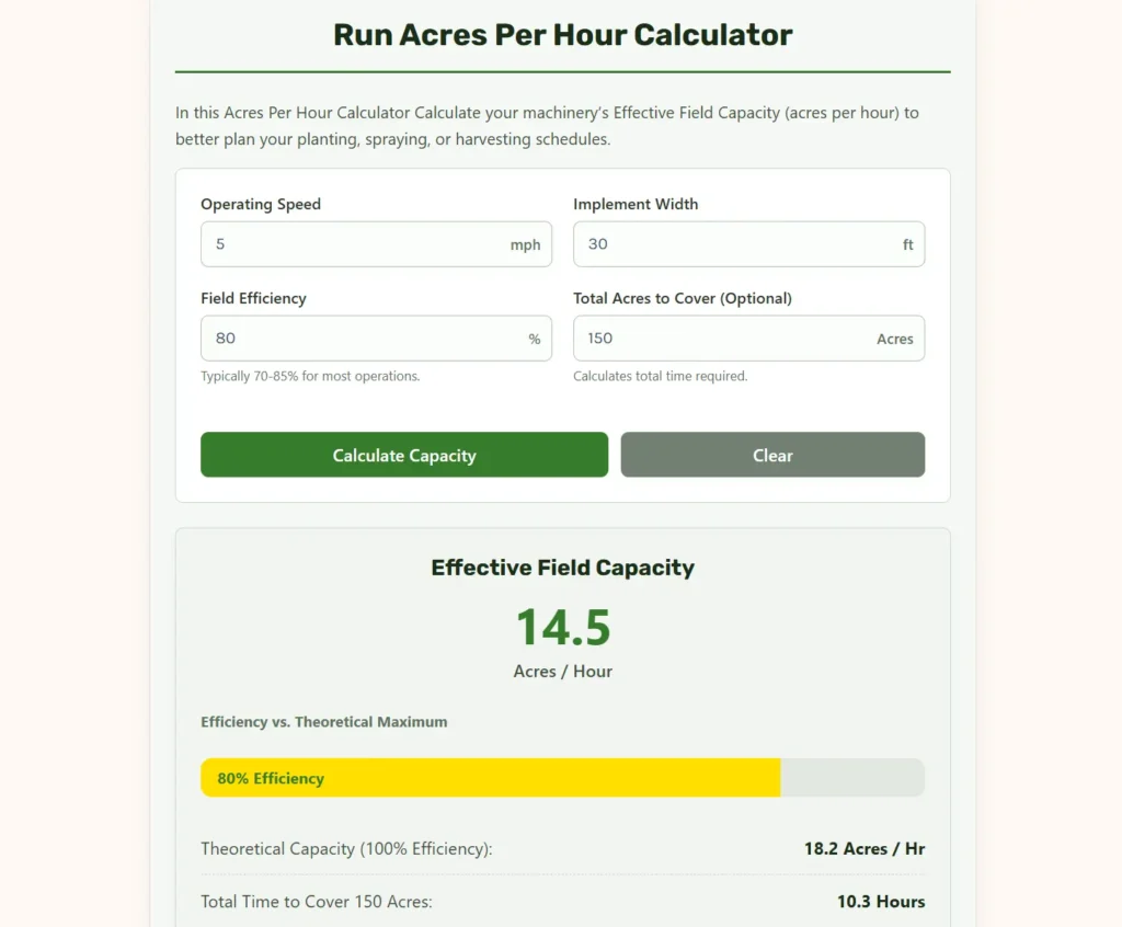
In this Acres Per Hour Calculator Calculate your machinery’s Effective Field Capacity (acres per hour) to better plan your planting, spraying, or harvesting schedules.
How It’s Calculated
The Field Capacity Formula
The standard agricultural formula uses a constant of 8.25. This constant is derived by dividing the square feet in a mile (5,280 ft) by the square feet in an acre (43,560 sq ft).
Understanding Field Efficiency
Theoretical Field Capacity assumes your machinery operates at a constant speed, using 100% of its width, with absolutely no stops. This is mathematically impossible in the real world.
Effective (Practical) Capacity accounts for real-world delays, represented as a percentage (Efficiency). Common causes for reduced efficiency include:
- Turning around at the ends of rows (headlands).
- Overlapping passes to ensure full coverage.
- Stopping to refill seed, fertilizer, or spray tanks.
- Unloading harvested crops on the go or while stopped.
- Minor adjustments or unclogging machinery.
Optimizing Field Capacity: The Science and Mathematics of Acres Per Hour
Modern agricultural economics operate on narrow profit margins, where operational success is heavily dependent on execution timing. Whether managing planting, chemical application, or harvesting, agricultural operators must work within brief, unpredictable weather windows. If a crop is planted too late or harvested past its peak moisture profile, the resulting yield penalties can directly impact seasonal profitability.
To manage these tight timelines, agricultural managers must treat machinery throughput not as a matter of estimation, but as a precise engineering calculation. This Acres Per Hour Calculator functions as a technical bridge, allowing operators to convert the physical parameters of their machinery—implement width, operating speed, and field efficiency—into a highly accurate metric known as Effective Field Capacity.
By understanding how these variables interact mathematically, operators can plan daily logistics, size tractor fleets, and optimize fuel and labor allocation with absolute certainty.
Defining Field Capacity: Theoretical vs. Effective
To calculate machinery throughput, we must first distinguish between the theoretical limits of a machine and its actual, real-world performance. In agricultural engineering, this distinction is defined by two key metrics:
1. Theoretical Field Capacity (TFC)
This represents the maximum rate of area coverage if the machine is operating at $100\%$ of its rated width, $100\%$ of the time, at a constant, uninterrupted forward speed. TFC assumes a perfect, endless field with no turning at row ends, no equipment overlaps, and no stops to refill consumables such as seed, fertilizer, or fuel.
2. Effective Field Capacity (EFC)
This is the actual rate of coverage achieved in practice under real-world field conditions. EFC factors in inevitable operational delays, including headland turns, refilling pauses, grain tank unloading, and operator overlapping.
The ratio between these two metrics is known as Field Efficiency, expressed as:$$\eta = \frac{C_e}{C_t}$$
Variable Definitions:
➜ $\eta$: The field efficiency of the operation, expressed as a decimal value.
➜ $C_e$: The Effective Field Capacity of the implement (acres per hour).
➜ $C_t$: The Theoretical Field Capacity of the implement (acres per hour).
The Mathematical Engine: Deriving the “8.25” Constant
A common point of confusion for operators is the origin of the constant $8.25$ used in the standard field capacity equation. To establish the mathematical validity of this tool, we must perform a complete dimensional analysis.
The objective is to calculate the area covered in acres per hour ($ac/hr$) using speed measured in miles per hour ($mph$) and implement width measured in feet ($ft$).
Step A: Determine Distance Covered in One Hour
If a tractor travels at a speed of $S$ miles per hour, the physical distance covered in one hour, expressed in feet, is:$$\text{Distance} = S \text{ miles} \times 5,280 \text{ feet/mile}$$
Variable Definitions:
➜ $\text{Distance}$: The linear distance traveled by the machinery in one hour (feet).
➜ $S$: The forward operating speed of the machinery (miles per hour).
➜ $5,280$: The physical constant representing the number of linear feet in one mile.
Step B: Determine the Area Covered in Square Feet
Assuming the implement uses its full rated width ($W$) in feet, the total area swept by the machine in one hour, expressed in square feet, is:$$\text{Area}_{\text{sq ft}} = (S \times 5,280) \text{ feet} \times W \text{ feet}$$
Variable Definitions:
➜ $\text{Area}_{\text{sq ft}}$: The total two-dimensional area swept by the implement in one hour (square feet).
➜ $S$: The operating speed (miles per hour).
➜ $W$: The physical working width of the implement (feet).
Step C: Convert Square Feet to Acres
Since one acre of land is defined as exactly $43,560 \text{ square feet}$, we convert the area from square feet to acres by dividing by this constant:$$\text{Area}_{\text{acres}} = \frac{S \times 5,280 \times W}{43,560}$$
Variable Definitions:
➜ $\text{Area}_{\text{acres}}$: The total area covered by the implement in one hour (acres).
➜ $S$: The operating speed (miles per hour).
➜ $W$: The working width of the implement (feet).
Step D: Simplify the Algebraic Fraction
To simplify the equation for field operators, we can divide both the numerator and the denominator by $5,280$:$$\text{Constant} = \frac{43,560}{5,280} = 8.25$$
This algebraic simplification yields the standard Theoretical Field Capacity formula used globally by agricultural engineers:$$C_t = \frac{S \times W}{8.25}$$
Variable Definitions:
➜ $C_t$: The Theoretical Field Capacity (acres per hour).
➜ $S$: The forward operating speed (miles per hour).
➜ $W$: The working width of the implement (feet).
➜ $8.25$: The derived unit conversion constant, carrying the units of $(\text{mile-foot})/\text{acre}$.
Calculating Effective Field Capacity
To transition from theoretical output to practical, real-world projections, we must integrate Field Efficiency ($\eta$) into the mathematical engine.$$C_e = \frac{S \times W \times \eta}{8.25}$$
Variable Definitions:
➜ $C_e$: The Effective Field Capacity (acres per hour).
➜ $S$: The forward operating speed (miles per hour).
➜ $W$: The working width of the implement (feet).
➜ $\eta$: The field efficiency of the operation, expressed as a decimal value (for example, $0.80$ represents $80\%$ efficiency).
➜ $8.25$: The unit conversion constant.
Calculating Total Operational Time
If an operator knows the total acreage of the target fields, they can use the Effective Field Capacity to calculate the exact number of hours required to complete the operation:$$T_{\text{total}} = \frac{A}{C_e}$$
Variable Definitions:
➜ $T_{\text{total}}$: The total operational time required to complete the work (hours).
➜ $A$: The total land area of the fields (acres).
➜ $C_e$: The calculated Effective Field Capacity (acres per hour).
Factors Influencing Field Efficiency
Field efficiency is never $100\%$. Under real-world conditions, efficiency fluctuates based on equipment type, field shape, operator experience, and tender logistics.
       [ Total Scheduled Field Time ]
                     |
       +-------------+-------------+
       |                           |
[ Productive Time ]         [ Idle Time (Losses) ]
  (Actual Field work)              |
                    +--------------+--------------+
                    |                             |
             [ Spatial Losses ]           [ Logistics Losses ]
             - Headland Turns             - Seed/Chemical Refills
             - Overlapping Passes         - Grain Tank Unloading
             - Avoiding Obstacles         - Mechanical Adjustments
The primary sources of efficiency loss in agricultural operations include:
➜ Headland Turning Patterns
When a tractor reaches the edge of a field (the headland), the operator must raise the implement, turn the machine $180$ degrees, align it with the next pass, and lower the implement back into the soil. During this turning loop, the machine is consuming fuel and labor without covering any productive acreage.
➜ Overlapping and Steering Errors
Without automated guidance systems, human operators tend to overlap their passes slightly to ensure no strips of unworked soil or untreated crop are left behind. Every foot of overlap directly reduces the effective working width of the implement, dragging down the overall field capacity.
➜ Material Handling and Refilling Logistics
Planters, seed drills, and sprayers must stop periodically to refill their hoppers or tanks. The time spent driving to the field edge, waiting for the tender truck, and loading product is a major source of idle time.
➜ Unloading Protocols
Combine harvesters must stop to empty their grain tanks once full unless they utilize a “grain cart” system to unload on-the-go. Stopping to unload can easily drop a harvesting operation’s efficiency below $65\%$.
Standard ASABE Field Efficiency Benchmarks
The American Society of Agricultural and Biological Engineers (ASABE) compiles empirical data on machinery performance. The table below represents standard speeds and efficiencies for common field operations:
| Implement Category | Speed Range (mph) | Typical Efficiency (%) | Primary Time Loss Drivers |
| Moldboard Plow | $3.5 – 6.0$ | $70 – 90\%$ | Row-end turning, soil obstructions |
| Chisel Plow / Disk | $4.0 – 6.5$ | $75 – 90\%$ | Turning, overlapping on odd-shaped fields |
| Row Crop Planter | $4.5 – 7.5$ | $65 – 85\%$ | Refilling seed/fertilizer, calibration |
| Grain Drill (Small Grain) | $4.0 – 6.5$ | $65 – 80\%$ | Refilling seed, cleaning disc openers |
| Boom Sprayer | $10.0 – 20.0$ | $60 – 75\%$ | Refilling water/pesticide, folding boom |
| Combine (Corn/Soybeans) | $3.0 – 5.0$ | $65 – 80\%$ | Unloading grain tank, clearing residue |
| Combine (Small Grains) | $3.0 – 4.5$ | $70 – 85\%$ | Unloading, slower speeds in high straw |
| Mower Conditioner | $5.0 – 8.5$ | $75 – 90\%$ | Turning, clearing heavy crop blockages |
Practical Step-by-Step Sizing Scenarios
To demonstrate how these calculations are applied on a commercial scale, let us analyze two common field management scenarios.
Scenario A: High-Speed Planting Operation
A corn grower in Iowa is planning their spring planting schedule. They want to determine if their 24-row planter can finish a 1,200-acre tract within a 3-day weather window.
- Implement Working Width ($W$): 24 rows with 30-inch spacing.
$$W = \frac{24 \times 30 \text{ in}}{12 \text{ in/ft}} = 60 \text{ ft}$$ - Operating Speed ($S$): $5.5 \text{ mph}$
- Target Field Efficiency ($\eta$): $75\%$ ($0.75$) based on typical seed tender logistics.
- Total Area ($A$): $1,200 \text{ acres}$
➜ Step 1: Calculate the Theoretical Field Capacity ($C_t$):$$C_t = \frac{5.5 \times 60}{8.25} = 40.0 \text{ acres/hour}$$
➜ Step 2: Calculate the Effective Field Capacity ($C_e$):$$C_e = 40.0 \times 0.75 = 30.0 \text{ acres/hour}$$
➜ Step 3: Calculate the total hours required to finish the tract:$$T_{\text{total}} = \frac{1,200}{30.0} = 40 \text{ Hours of operation}$$
If the grower operates 14 hours per day, the job will take approximately $2.86$ days. This confirms that their current machinery setup can safely complete the planting before the weather window closes.
Scenario B: High-Throughput Combine Harvesting
A wheat grower in Kansas is harvesting a standard section of land ($640 \text{ acres}$) using a modern combine harvester.
- Implement Working Width ($W$): $40 \text{ ft}$ grain platform.
- Operating Speed ($S$): $4.2 \text{ mph}$
- Field Efficiency ($\eta$): $70\%$ ($0.70$) because they are unloading into static semi-trucks parked at the field edge.
- Total Area ($A$): $640 \text{ acres}$
➜ Step 1: Calculate the Theoretical Field Capacity ($C_t$):$$C_t = \frac{4.2 \times 40}{8.25} \approx 20.36 \text{ acres/hour}$$
➜ Step 2: Calculate the Effective Field Capacity ($C_e$):$$C_e = 20.36 \times 0.70 \approx 14.25 \text{ acres/hour}$$
➜ Step 3: Calculate the total hours required to harvest the section:$$T_{\text{total}} = \frac{640}{14.25} \approx 44.91 \text{ Hours of operation}$$
Assuming 10 hours of optimal dry harvesting sunlight per day, this harvest will take $4.5$ days to complete. If the grower wants to speed up this timeline, they could add a grain cart to unload on-the-go, raising their efficiency to $85\%$ and reducing the required time to $37$ hours ($3.7$ days).
Best Practices to Maximize Field Efficiency
To minimize idle time and get the most out of your machinery investment, consider these industry-proven practices:
- Implement RTK GPS Auto-Steer: Using Real-Time Kinematic (RTK) automated steering reduces overlaps down to less than one inch. This permanently preserves the full working width of the implement and reduces operator fatigue.
- Synchronize Grain Cart Logistics: In harvesting operations, keeping a dedicated tractor and grain cart running alongside the combine allows the combine to unload on-the-go. This simple logistical change can raise combine efficiency from $65\%$ to over $85\%$.
- Optimize Headland Width and Turn Styles: Make sure headlands are wide enough to allow for continuous turning loops. For larger implements, a “keyhole” or “loop” turn is often faster and causes less soil compaction than backing up to make a three-point turn.
- Pre-Position Tender Vehicles: Position seed and chemical tenders strategically at the field boundary. If you have irregular or very long fields, placing tenders at both ends can significantly reduce travel time when tanks run empty.
- Track Machine Maintenance Schedules: Check disc openers, grease fittings, and sprayer nozzles before heading to the field. Stopping to replace a clogged nozzle or broken shear bolt in the middle of a tight planting window directly impacts seasonal field capacity.
Technical Definitions and Glossary
➜ Effective Field Capacity: The actual average rate of land coverage achieved by a machine, factoring in all turning, overlapping, and maintenance delays.
➜ Field Efficiency: The ratio of effective field capacity to theoretical field capacity, reflecting how well-organized the operation is.
➜ Gunter’s Chain: A historical surveying tool equal to $66 \text{ feet}$, used to establish standard agricultural area measurements.
➜ Headlands: The strips of land at the ends of a field where machinery turns around. These are typically worked last, after the main rows are completed.
➜ Implement Width: The physical working width of an implement (such as a planter or disk), measured perpendicular to the direction of travel.
➜ Overlapping: The practice of re-working a small portion of a previous pass to ensure complete coverage, which reduces the effective width of the machine.
➜ Theoretical Field Capacity: The maximum rate of area coverage a machine could theoretically achieve if it ran continuously at full speed and width.
Scientific Reference and Empirical Standards
The logic and constants used in agricultural machinery management are governed by the standards set by the leading global authority on agricultural engineering.
Relevance: This engineering standard provides the foundational guidelines, draft formulas, and field efficiency tables used by machinery designers and farm managers globally. The calculations for theoretical and effective field capacity in this guide are derived from ASABE’s standardized methodologies, ensuring that the results are fully compatible with professional fleet planning, university extension research, and commercial farm software.
Final Summary Checklist for Farm Managers
Before deploying machinery for your next major field operation, run through this final logistical checklist:
✓ Is your forward operating speed matched to the soil conditions and the tractor’s horsepower (draft requirements)?
✓ Have you calculated the working width of your implement in feet, taking any necessary overlaps into account?
✓ Have you selected a realistic Field Efficiency benchmark based on your current support staff and tender logistics?
✓ If you have entered a total target acreage, does the calculated time fit within your local weather window?
✓ Have you planned a turning pattern at the headlands that minimizes soil compaction and idle time?
By utilizing this Acres Per Hour Calculator and applying these structured operational guidelines, you can transition from speculative scheduling to precise, data-driven farm management. Maximizing your acres per hour is the primary safeguard against weather risks and the foundation of a highly profitable, modern agricultural business.