Use Present Value of Annuity Calculator
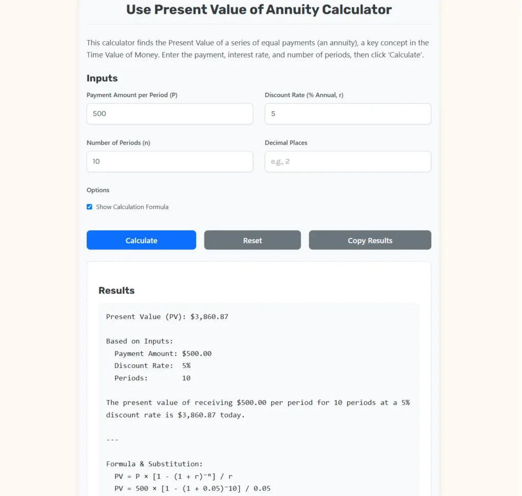
This calculator finds the Present Value of a series of equal payments (an annuity), a key concept in the Time Value of Money. Enter the payment, interest rate, and number of periods, then click ‘Calculate’.
Inputs
Explanation
The Present Value of an Annuity tells you the total worth of a stream of equal, regular payments in today’s money. This is essential for comparing investments, valuing loans, and planning for retirement. It works by “discounting” each future payment back to its present-day value.
Formula
The formula to calculate the Present Value of an ordinary annuity is: PV = P × [1 - (1 + r)⁻ⁿ] / r
Worked Example
What is the present value of receiving $500 annually for 10 years if the annual discount rate is 5%?
- Payment (P) =
$500 - Discount Rate (r) =
0.05(5%) - Periods (n) =
10
PV = 500 × [1 - (1 + 0.05)⁻¹⁰] / 0.05 = 3,860.87
This means receiving 500 every year for 10 years is worth 3,860.87 to you today if your discount rate is 5%.
Present Value of Annuity: Financial Mechanics, Mathematical Foundations, and Valuation Strategies
Evaluating fixed-interval payment streams represents a core discipline across corporate finance, actuarial science, wealth management, and capital allocation. The Present Value of an Annuity (PVA) quantifies today’s aggregate monetary worth of a series of equal cash inflows or outflows received or paid at regular future intervals.
Because money available today can earn compound interest, and because general price inflation erodes purchasing power over time, a dollar scheduled for receipt in the future possesses less financial value than a dollar held today. The Present Value of Annuity Calculator converts extended payment schedules into a single baseline valuation figure, allowing investors, financial planners, and corporate officers to compare structured payment streams against immediate lump-sum alternatives on an equivalent footing.
+-----------------------------------------------------------------------+
|                 PRESENT VALUE OF ANNUITY (PVA) FLOW                   |
|                                                                       |
|   Payment (P) Period 1  ➔  Discount Factor: (1+r)^-1  ➔  Today's $    |
|   Payment (P) Period 2  ➔  Discount Factor: (1+r)^-2  ➔  Today's $    |
|   Payment (P) Period n  ➔  Discount Factor: (1+r)^-n  ➔  Today's $    |
|                                                                       |
|   Consolidated Output: Total Present Value (PV) Sum                   |
+-----------------------------------------------------------------------+
Fundamental Economic Concepts of Annuity Valuation
An annuity is defined as a financial structure featuring a sequence of identical payments occurring at regular, equal time intervals across a finite duration. Annuity valuation relies upon three structural variables:
- Periodic Payment Magnitude (P): The fixed nominal monetary sum disbursed or received during each individual payment cycle.
- Discount Rate per Period (r): The opportunity cost of capital or required rate of return expressed as a decimal fraction per compounding interval.
- Total Number of Periods (n): The aggregate count of payment intervals throughout the lifetime of the financial contract.
Time Value of Money and Discounting Mechanics
Discounting reverses the process of compound interest expansion. While future value compounding determines how capital expands forward across time, present value discounting calculates the lump-sum investment required today at rate r to replicate every scheduled future payment exactly when due.
Compounding (Forward Growth):  Present Value (PV) ➔ Compound Engine ➔ Future Value (FV)
Discounting (Backward Value):  Future Cash Streams ➔ Discount Engine ➔ Present Value (PV)
As the discount rate r increases, the present value of future annuity payments declines because each dollar invested today generates a higher yield, requiring less initial principal to meet future obligation targets.
Mathematical Foundations and Formula Derivations
The total present value of an ordinary annuity equals the algebraic sum of the individual present values of all future payments across periods t = 1 to n.
Discrete Summation Representation
Expressing the annuity sum explicitly produces the polynomial series:
PV = [ P / (1 + r)1 ] + [ P / (1 + r)2 ] + [ P / (1 + r)3 ] + … + [ P / (1 + r)n ]
Factoring out the constant payment term P yields:
PV = P × ∑t=1n [ 1 / (1 + r)t ]
Closed-Form Formula Derivation via Geometric Series
Calculating individual discounted periods manually for long-term annuities is computationally inefficient. Applying the finite geometric series summation identity compresses the discrete summation into a single closed-form equation.
Let the Present Value Interest Factor of an Annuity (PVIFA) be represented as:
PVIFAr, n = ∑t=1n (1 + r)−t
Multiplying both sides by (1 + r) produces:
(1 + r) × PVIFA = ∑t=1n (1 + r)1−t = 1 + (1 + r)−1 + (1 + r)−2 + … + (1 + r)−(n−1)
Subtracting the original PVIFA equation from this expanded expression cancels all intermediate terms, leaving:
r × PVIFA = 1 − (1 + r)−n
Dividing by the periodic discount rate r produces the standard closed-form Annuity Factor equation:
PVIFAr, n = [ 1 − (1 + r)−n ] / r
Multiplying this factor by the period payment magnitude P establishes the universal Ordinary Annuity Present Value formula:
PV = P × [ 1 − (1 + r)−n ] / r
+-----------------------------------------------------------------------+
|                    CLOSED-FORM PVA FORMULA                            |
|                                                                       |
|               1 - (1 + r)^(-n)                                        |
|   PV =  P * --------------------                                      |
|                      r                                                |
|                                                                       |
|   Where:                                                              |
|   PV = Present Value of the Ordinary Annuity                          |
|   P  = Fixed Payment per Period                                       |
|   r  = Discount Rate per Period (Decimal Format)                      |
|   n  = Total Number of Compounding Periods                            |
+-----------------------------------------------------------------------+
Limiting Case: Perpetuities (Infinite Duration)
When the payment duration extends infinitely toward mathematical infinity (n → ∞), the exponent term (1 + r)−n approaches zero. The closed-form equation simplifies to the classic Perpetuity Formula:
PVperpetuity = P / r
This asymptotic relationship underpins perpetual bond valuation, preferred stock dividend pricing, and real estate capitalization rate models.
Ordinary Annuity versus Annuity Due Structure
Financial contracts specify distinct payment timing schedules. Distinguishing between ordinary annuities and annuities due is essential for avoiding valuation errors.
Ordinary Annuity Timeline (End of Period):
Period 0 --------------- Period 1 --------------- Period 2 --------------- Period 3
                            [ $P ]                   [ $P ]                   [ $P ]

Annuity Due Timeline (Beginning of Period):
Period 0 --------------- Period 1 --------------- Period 2 --------------- Period 3
   [ $P ]                   [ $P ]                   [ $P ]
1. Ordinary Annuity
In an ordinary annuity structure, cash flows occur at the end of each compounding period. Standard retail loans, corporate bond coupon payments, and consumer mortgages function as ordinary annuities. The first payment experiences one full compounding period of discounting.
2. Annuity Due
In an annuity due structure, cash flows occur at the beginning of each compounding period. Real estate lease agreements, equipment rentals, and insurance premium payments function as annuities due. Because every cash flow occurs one period earlier relative to an ordinary annuity, each payment experiences one less period of discounting.
To convert an ordinary annuity present value into an annuity due present value, multiply the standard result by (1 + r):
PVdue = PVordinary × (1 + r)
PVdue = P × [ 1 − (1 + r)−n ] × (1 + r) / r
Structural Comparison Matrix
| Metric Feature | Ordinary Annuity | Annuity Due |
| Payment Timing | End of each period | Beginning of each period |
| First Payment Discounting | Discounted by 1 period: (1+r)−1 | Not discounted: (1+r)0 = 1 |
| Relative Present Value | Lower valuation baseline | Higher valuation baseline by factor of (1+r) |
| Primary Real-World Examples | Corporate bonds, mortgages, consumer loans | Commercial leases, insurance premiums, equipment hires |
Architecture and Algorithmic Execution of the Calculator Engine
Modern digital conversion engines compute annuity valuations by processing user input parameters through normalization pipelines, numerical constraint checks, and formatting routines.
                  +-----------------------------------+
                  |  ANNUITY CALCULATOR ENGINE FLOW   |
                  +-----------------------------------+
                                    |
                                    v
                         +--------------------+
                         | PARSE USER INPUTS  |
                         | P, r_input, n      |
                         +--------------------+
                                    |
                                    v
                         +--------------------+
                         | VALIDATE BOUNDS    |
                         | P > 0, r > 0, n > 0|
                         +--------------------+
                                    |
                                    v
                         +--------------------+
                         | NORMALIZE RATE     |
                         | r = r_input / 100  |
                         +--------------------+
                                    |
                                    v
                         +--------------------+
                         | COMPUTE PVIFA      |
                         | [1-(1+r)^-n] / r   |
                         +--------------------+
                                    |
                                    v
                         +--------------------+
                         | MULTIPLY FACTOR    |
                         | PV = P * PVIFA     |
                         +--------------------+
                                    |
                                    v
                         +--------------------+
                         | FORMAT OUTPUT      |
                         | Rounding & Currency|
                         +--------------------+
Algorithmic Execution Steps
- Input Parsing and Normalization: Read user form entries for payment magnitude P, nominal annual discount rate rinput, and period count n. Convert percentage rate inputs to decimal format: r = rinput / 100. If the user enters a decimal fraction directly (0 < rinput < 1), normalize it directly to avoid double scaling.
- Validation and Singularity Checks: Verify that P > 0, n > 0, and r > 0. If r = 0, bypass exponent calculation to prevent division-by-zero errors, applying the linear fallback identity: PV = P × n.
- Present Value Factor Computation: Calculate exponential growth term: Term = (1 + r)−n. Subtract from unity: Numerator = 1 − Term. Divide by period rate: PVIFA = Numerator / r.
- Total Valuation Synthesis: Compute final product: PV = P × PVIFA.
- Step-by-Step Substitution Construction: If formula transparency is toggled, build an explicit step-by-step mathematical output displaying intermediary products, rates, and factors to facilitate manual auditing.
- Precision Rendering: Apply user-selected decimal rounding (typically 2 decimal places for financial reporting) and format strings into standard ISO currency representations.
Step-by-Step Worked Mathematical Examples
Example 1: Evaluating a 10-Year Retirement Income Annuity
A financial planner evaluates an ordinary annuity offering equal annual payouts of $500.00 for 10 years. The client applies an annual discount rate of 5.00%.
- Input Parameters:
- Periodic Payment (P) = $500.00
- Discount Rate (r) = 5.00% = 0.05
- Period Count (n) = 10 years
Step A: Calculate Exponential Discounting Denominator
(1 + r)−n = (1 + 0.05)−10 = (1.05)−10 = 0.613913
Step B: Determine the Present Value Interest Factor (PVIFA)
Numerator = 1 − 0.613913 = 0.386087
PVIFA0.05, 10 = 0.386087 / 0.05 = 7.721735
Step C: Synthesize Aggregate Present Value
PV = $500.00 × 7.721735 = $3,860.87
Summary Breakdown for Example 1:
| Period (t) | Nominal Payment (P) | Discount Factor (1+r)−t | Discounted Present Value | Cumulative PV |
| Year 1 | $500.00 | 0.952381 | $476.19 | $476.19 |
| Year 2 | $500.00 | 0.907029 | $453.51 | $929.70 |
| Year 3 | $500.00 | 0.863838 | $431.92 | $1,361.62 |
| Year 4 | $500.00 | 0.822702 | $411.35 | $1,772.97 |
| Year 5 | $500.00 | 0.783526 | $391.76 | $2,164.73 |
| Year 6 | $500.00 | 0.746215 | $373.11 | $2,537.84 |
| Year 7 | $500.00 | 0.710681 | $355.34 | $2,893.18 |
| Year 8 | $500.00 | 0.676839 | $338.42 | $3,231.60 |
| Year 9 | $500.00 | 0.644609 | $322.30 | $3,553.90 |
| Year 10 | $500.00 | 0.613913 | $306.96 | $3,860.87 |
Although the cumulative nominal sum of payments across ten years is 5,000.00, discounting at 5% reveals that the true value of this income stream today is 3,860.87.
Example 2: Commercial Real Estate Lease Evaluation (Annuity Due)
A real estate firm evaluates a five-year commercial lease contract requiring annual payments of $12,000.00 paid at the beginning of each year. The hurdle rate is set at 7.50%.
- Input Parameters:
- Payment (P) = $12,000.00
- Discount Rate (r) = 7.50% = 0.075
- Periods (n) = 5 years
Step A: Compute Ordinary Annuity Factor
(1.075)−5 = 0.696559
PVIFAordinary = (1 − 0.696559) / 0.075 = 0.303441 / 0.075 = 4.045880
Step B: Compute Ordinary Annuity Present Value
PVordinary = $12,000.00 × 4.045880 = $48,550.56
Step C: Adjust for Annuity Due Timing Offset
PVdue = PVordinary × (1 + r)
PVdue = $48,550.56 × 1.075 = $52,191.85
Paying at the start of each period increases the landlord’s present valuation by $3,641.29 compared to end-of-period payments.
Discount Rate Calibration and Market Factors
Selecting an accurate discount rate r is critical in financial modelling. Because r sits in the denominator of the discounting factor, adjustments to rate inputs exert a non-linear effect on present value outputs.
Rate Dynamics Matrix:
Higher Discount Rate (r ↑)  ➔  Smaller PVIFA Factors  ➔  Lower Present Value (PV ↓)
Lower Discount Rate (r ↓)   ➔  Larger PVIFA Factors   ➔  Higher Present Value (PV ↑)
Rate Selection Frameworks
- Weighted Average Cost of Capital (WACC): Used by corporations evaluating capital expenditure projects, lease arrangements, or internal asset investments. WACC incorporates both debt and equity financing costs.
- Risk-Free Rate plus Risk Premium: Used by portfolio managers, combining benchmark sovereign yields (such as 10-year US Treasury bonds) with a specific credit, liquidity, and default risk spread.
- Inflation-Adjusted Real Discount Rate: Applied during long-term financial planning to separate inflation purchasing power decay from real capital productivity.
Sensitivity Analysis: PVA Factors Across Differing Rates
The table below illustrates how changes in the discount rate r alter the Present Value Interest Factor of an Annuity (PVIFA) across varying durations.
| Period Count (n) | r = 3.0% | r = 5.0% | r = 8.0% | r = 10.0% | r = 12.0% |
| 5 Years | 4.5797 | 4.3295 | 3.9927 | 3.7908 | 3.6048 |
| 10 Years | 8.5302 | 7.7217 | 6.7101 | 6.1446 | 5.6502 |
| 15 Years | 11.9379 | 10.3797 | 8.5595 | 7.6061 | 6.8109 |
| 20 Years | 14.8775 | 12.4622 | 9.8181 | 8.5136 | 7.4694 |
| 30 Years | 19.6004 | 15.3725 | 11.2578 | 9.4269 | 8.0552 |
As period duration lengthens, present value factors exhibit diminishing marginal increases due to exponential compounding decay in distant cash flows.
Comprehensive Comparison of TVM Valuation Metrics
Present value of annuity mechanics exist within a broader ecosystem of Time Value of Money (TVM) metrics.
                  +-----------------------------------+
                  |      CORE TVM METRICS MATRIX      |
                  +-----------------------------------+
                                    |
         +--------------------------+--------------------------+
         |                                                     |
         v                                                     v
+------------------+                                 +------------------+
| STREAM VALUES    |                                 | SINGLE VALUES    |
| PVA: Equal Series|                                 | PV: Single Future|
| FVA: Compound Sum|                                 | FV: Compound End |
+------------------+                                 +------------------+
| Metric Name | Mathematical Definition | Financial Objective | Primary Use Case |
| Present Value of Annuity (PVA) | P × [ 1 − (1 + r)−n ] / r | Measures today’s single equivalent value of a future regular payment stream | Valuing pension payouts, lease obligations, loan principal |
| Future Value of Annuity (FVA) | P × [ (1 + r)n − 1 ] / r | Measures terminal accumulated wealth resulting from recurring deposits | Retirement savings projections, sinking fund accumulation |
| Present Value of Single Sum (PV) | CF / (1 + r)n | Measures today’s value of an isolated individual future cash flow | Zero-coupon bond pricing, terminal lump-sum valuation |
| Perpetuity Present Value | P / r | Measures today’s value of an infinite continuous payment stream | Preferred stock evaluation, endowment fund management |
Practical Industry Applications and Commercial Use Cases
                  +-----------------------------------+
                  |   COMMERCIAL INDUSTRY APPLICATIONS|
                  +-----------------------------------+
                                    |
         +--------------------------+--------------------------+
         |                                                     |
         v                                                     v
+------------------+                                 +------------------+
| REAL ESTATE LEASES|                                | CORPORATE BONDS  |
| Capitalization & |                                 | Coupon Stream    |
| Present Value    |                                 | Discounting      |
+------------------+                                 +------------------+
         |                                                     |
         v                                                     v
+------------------+                                 +------------------+
| RETIREMENT INCOME|                                 | CONSUMER LOANS   |
| Pension Drawdown |                                 | Amortization     |
| Modeling         |                                 | Schedules        |
+------------------+                                 +------------------+
1. Consumer Loan and Mortgage Amortization
Bank lending operations utilize annuity formulas to structure equal monthly loan repayments. The total principal borrowed equals the present value of the borrower’s scheduled monthly annuity payments discounted at the loan contract interest rate.
2. Corporate Fixed-Income Pricing
Fixed-rate bond prices equal the combined sum of two separate TVM components:
- The present value of the recurring coupon payment annuity.
- The present value of the face value principal repayment at maturity.
Bond traders revalue these annuity streams continuously as prevailing market interest rates fluctuate.
3. Retirement and Structured Pension Income Planning
Actuaries and wealth managers project structured retirement drawdowns using annuity equations. Determining how much capital an individual must accumulate prior to retirement requires calculating the present value of their desired post-retirement monthly income stream.
4. Commercial Real Estate and Capital Lease Accounting
Under international accounting standards (such as IFRS 16 and ASC 842), corporations must record lease liabilities on balance sheets. Lessees calculate this liability by determining the present value of future minimum lease payments using the firm’s incremental borrowing rate.
User Interface and Interaction Best Practices for Financial Tools
Creating accessible, reliable financial web calculators requires focusing on mathematical transparency, robust input handling, and responsive interface controls.
+-------------------------------------------------------------+
|              BEST PRACTICES FOR FINANCIAL UI/UX             |
|                                                             |
| ✔ Implement explicit rate normalization (handling % vs dec).|
| ✔ Provide formula visibility toggles for manual auditing.    |
| ✔ Support plain-language summary outputs for non-experts.   |
| ✔ Include a single-click copy feature for client reports.   |
| ✔ Enforce input constraints against zero or negative values. |
+-------------------------------------------------------------+
Key Functional UI Features
- Rate Input Normalization: Software input fields should dynamically parse both percentage integers (e.g., entering “5” for 5%) and decimal fractions (e.g., entering “0.05” for 5%) to eliminate user input errors.
- Auditability and Step Visibility: Include an expandable calculation steps panel that exposes explicit mathematical substitution, intermediate factor calculations, and algebraic breakdowns for professional verification.
- Plain-Language Summaries: Pair numerical output cards with clear plain-language descriptions that translate raw figures into intuitive economic narratives.
- Clipboard Integration: Provide formatted plain-text copying capabilities, allowing financial advisors and analysts to paste calculated results directly into client communications, spreadsheets, or investment memos.
Frequently Asked Questions (FAQ)
What is the core difference between an ordinary annuity and an annuity due?
In an ordinary annuity, payments occur at the end of each period, whereas in an annuity due, payments occur at the beginning of each period. Because payments in an annuity due occur one period earlier, they experience less discounting, resulting in a higher present value than an ordinary annuity with identical terms.
How does an increase in the discount rate impact the Present Value of an Annuity?
An increase in the discount rate decreases the Present Value of an Annuity. Higher discount rates represent a higher opportunity cost of capital, increasing the discounting factor in the denominator and reducing today’s valuation of future cash flows.
What happens to the annuity present value equation if the discount rate equals zero?
If the discount rate is zero percent (r = 0), discounting ceases to reduce future cash flows. The present value equation simplifies to simple linear multiplication: PV = P × n. Digital calculators implement fallback checks to handle r = 0 directly, preventing division-by-zero errors.
Can this calculation handle monthly or quarterly payment intervals?
Yes. To evaluate monthly or quarterly payment streams, parameters must be converted to match the periodic frequency. Divide the nominal annual discount rate by the compounding frequency per year (e.g., r = Annual Rate / 12 for monthly payments) and multiply the total duration in years by the same compounding frequency (e.g., n = Years × 12).
Why is the Present Value of an Annuity lower than the total nominal sum of all payments?
The Present Value of an Annuity is lower than the nominal sum of payments because money received in the future cannot earn interest today. Discounting strips away the interest earning capacity across future periods, reducing nominal dollar amounts to their equivalent purchasing value in current terms.
Academic References and Authoritative Standards
- Brigham, E. F., & Ehrhardt, M. C. (2019). Corporate Finance: Linking Theory to Capital Allocation Decisions. 16th Edition. Cengage Learning.
- Bodie, Z., Kane, A., & Marcus, A. J. (2021). Investments. 12th Edition. McGraw-Hill Education.
- International Accounting Standards Board (IASB). IFRS 16: Leases. International Financial Reporting Standards Documentation.
- Financial Accounting Standards Board (FASB). Accounting Standards Codification Topic 842 (ASC 842): Leases.
- Damodaran, A. (2012). Investment Valuation: Tools and Techniques for Determining the Value of Any Asset. 3rd Edition. John Wiley & Sons.