Use Graphing Calculator
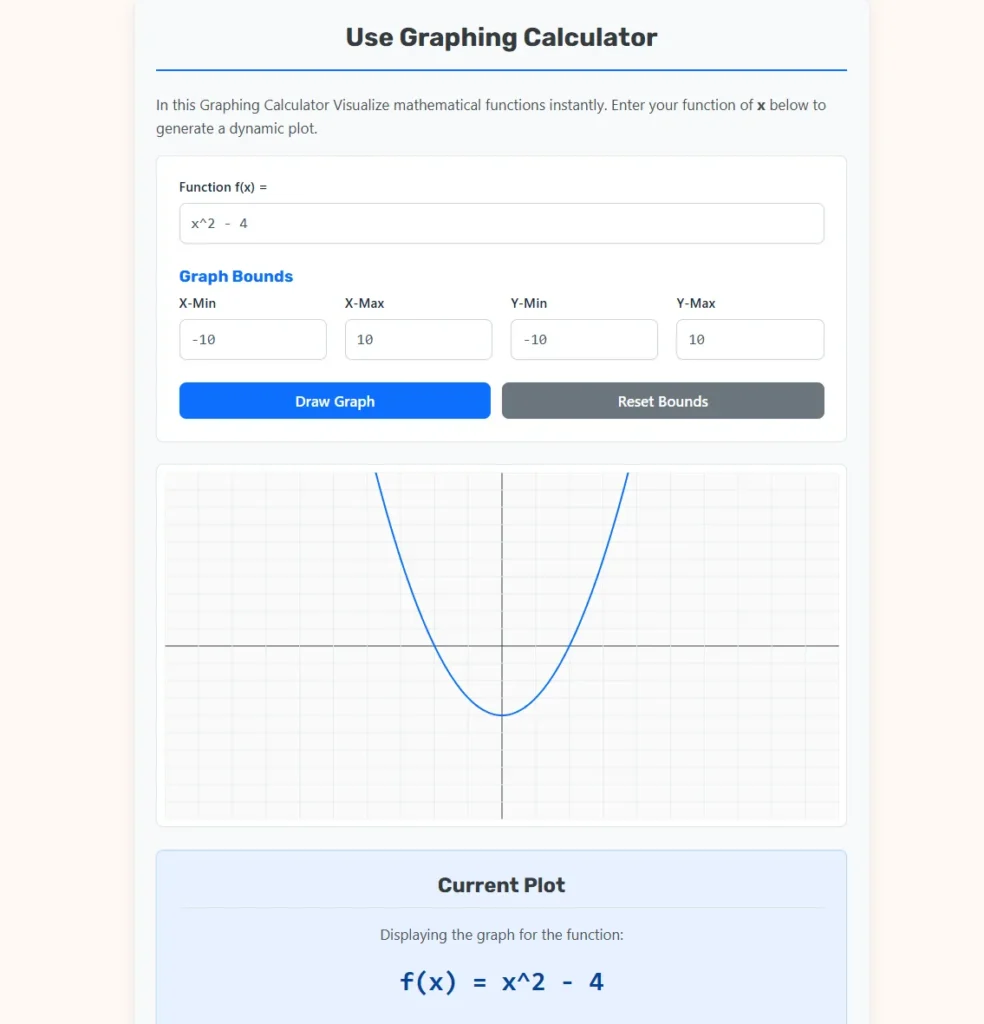
In this Graphing Calculator Visualize mathematical functions instantly. Enter your function of x below to generate a dynamic plot.
How to Write Equations
Use standard JavaScript math syntax or simple mathematical operators. Here are some examples of valid inputs:
- Basic Arithmetic:
x + 5,2 * x - 3 - Exponents: Use the caret symbol. Example:
x^2(x2) orx^3 - x(x3 – x). - Trigonometry:
sin(x),cos(x),tan(x). - Logarithms & Roots:
log(x)for natural log,sqrt(x)for square root. - Constants: Use
piore. Example:sin(x * pi). - Absolute Value:
abs(x).
Guide to Function Plotting and Analysis
Mathematics is often perceived as a collection of abstract rules and symbolic manipulations; however, the true power of mathematical thought is realized through visualization. The graphing of a function represents the translation of numerical relationships into spatial geometry. By plotting the values of a dependent variable against an independent variable on a Cartesian plane, we can observe patterns, identify critical behaviors, and predict future outcomes with structural clarity.
The Graphing Calculator serves as a high-fidelity rendering instrument designed to bridge the gap between algebraic theory and visual intuition. By deconstructing the behavior of functions—ranging from simple linear slopes to complex trigonometric oscillations—this tool provides users with an immediate window into the logic of the universe. This guide explores the mechanical foundations of coordinate systems, the geometric properties of various function families, and the diverse real-world applications where graphing is non-negotiable.
Defining the Cartesian Coordinate System
To utilize a graphing tool effectively, one must first understand the environment in which the data exists. The Cartesian coordinate system, developed by René Descartes in the 17th century, revolutionized mathematics by merging algebra and geometry.
$\rightarrow$ The X-Axis (Abscissa): The horizontal line representing the independent variable.
$\rightarrow$ The Y-Axis (Ordinate): The vertical line representing the dependent variable.
$\checkmark$ The Origin: The point $(0, 0)$ where the axes intersect.
$\checkmark$ The Quadrants: The four regions of the plane defined by the positive and negative directions of the axes.
$\checkmark$ The Bounds: The minimum and maximum visible limits of the grid, which determine the “window” through which the function is observed.
Mathematical Foundations: The Mechanics of the Plot
Behind the user interface of the calculator lies a sequence of iterative calculations. To render a curve, the tool evaluates the function at hundreds of discrete points along the x-axis and connects them with infinitesimal lines to simulate a continuous path.
1. The Mapping Transformation
To translate a mathematical result into a pixel on your screen, the calculator utilizes a linear mapping algorithm.
$$P_x = \frac{x – x_{min}}{x_{max} – x_{min}} \times W$$
- $P_x$: The specific pixel coordinate on the horizontal axis of the canvas.
- $x$: The mathematical value being evaluated.
- $x_{min}, x_{max}$: The user-defined horizontal boundaries.
- $W$: The total width of the rendering surface in pixels.
This formula ensures that regardless of the scale—whether observing the micro-movements of a quantum particle or the macro-orbits of a planet—the graph remains perfectly proportional within the display area.
2. The Functional Relationship
Every graph generated is a visual representation of a mapping from a domain to a range.
$$y = f(x)$$
- $y$: The output value or height on the vertical axis.
- $f$: The specific mathematical operation or set of operations.
- $x$: The input value within the established domain.
Analyzing Common Function Families
The diversity of the physical world is modeled through different “families” of functions. Each family possesses unique geometric signatures that reveal the nature of the relationship being studied.
Linear Functions: The Geometry of Constant Change
Linear functions are the simplest form of relationship, representing a constant rate of change. They appear as perfectly straight lines.
$$f(x) = mx + b$$
- $m$: The slope, representing the vertical rise over the horizontal run.
- $b$: The y-intercept, indicating the value of the function when $x$ is zero.
$\rightarrow$ Interpretation: A positive slope indicates growth, while a negative slope indicates decay. If the slope is zero, the relationship is constant.
Quadratic Functions: The Parabolic Path
Quadratic functions are second-degree polynomials that produce a curve known as a parabola. These are foundational in the study of physics and projectiles.
$$f(x) = ax^2 + bx + c$$
- $a$: Determines the concavity (opening upward if positive, downward if negative).
- $b$: Influences the horizontal position of the vertex.
- $c$: The y-intercept of the curve.
$\checkmark$ The Vertex: The absolute maximum or minimum point of the parabola.
$\checkmark$ Roots: The points where the parabola crosses the x-axis, found by solving the quadratic formula.
Trigonometric Functions: The Pulse of Periodicity
Trigonometric functions, such as Sine and Cosine, model cyclical or periodic behavior. These are essential for understanding sound waves, light, and alternating current.
$$f(x) = A \sin(B(x – C)) + D$$
- $A$: The amplitude, representing the height of the wave from the center.
- $B$: The frequency modifier, determining how many cycles occur over a distance.
- $C$: The phase shift, moving the wave horizontally.
- $D$: The vertical shift or baseline.
Industry Use Cases and Practical Applications
Graphing is not a purely academic exercise; it is a vital component of modern industry and scientific discovery.
1. Civil Engineering and Structural Analysis
Engineers use graphing to model the “Bending Moment” of beams in skyscrapers and bridges. By plotting the force applied against the length of the structure, they can identify the exact points of maximum stress. This visualization prevents structural failure by ensuring that reinforcement is placed exactly where the math predicts the highest load.
2. Economics and Market Equilibrium
In the financial sector, graphing is used to identify the “Break-even Point.” By plotting the total cost function against the total revenue function, analysts can see where the two lines intersect.
$\checkmark$ The Equilibrium Point: The intersection where supply equals demand.
$\checkmark$ The Margin of Safety: The area on the graph where revenue exceeds costs.
3. Epidemiology and Biological Modeling
Researchers use the “Logistic Growth Curve” (an S-shaped graph) to predict how a virus spreads through a population or how a specific species will populate an ecosystem.
$\rightarrow$ The Carrying Capacity: The upper asymptote of the graph where growth stabilizes due to environmental limits.
4. Computer Graphics and Game Development
Modern video games rely on “Bezier Curves” and functional plotting to manage character movement and lighting. When a character jumps, the path they follow is often a real-time plot of a quadratic function processed by the game engine.
Advanced Operators and Syntax Rules
To unlock the full potential of the Graphing Calculator, one must utilize the correct syntax for complex operations.
| Mathematical Goal | Required Syntax | Example |
| Square Roots | sqrt(x) | sqrt(x^2 + 1) |
| Absolute Value | abs(x) | abs(x - 5) |
| Natural Logarithm | log(x) | log(x) * 2 |
| Exponents | x^n or x**n | x^3 - 2*x |
| Constants | pi or e | sin(x * pi) |
$\rightarrow$ Order of Operations: The calculator follows the standard algebraic hierarchy (Parentheses, Exponents, Multiplication/Division, Addition/Subtraction). Always use parentheses to clarify complex numerators or denominators.
Interpreting Graph Results: Critical Features
When a graph is rendered, the expert observer looks for specific features that define the function’s character.
- Intercepts: Points where the graph crosses the axes. The x-intercepts are the “zeros” or “solutions” to the equation.
- Symmetry: Does the graph look the same when flipped over the y-axis (Even function) or rotated around the origin (Odd function)?
- Asymptotes: Lines that the graph approaches but never touches. These often indicate “limits” or undefined values in the function (such as dividing by zero).
- Extrema: The peaks (local maxima) and valleys (local minima) of the curve. These are critical in optimization problems.
Best Practices for Optimal Visualization
To ensure the most useful data representation, adhere to the following professional standards:
$\checkmark$ Adjust Your Bounds: If a parabola appears as a straight line, your X-Min and X-Max might be too narrow. If the graph disappears, your Y-bounds may not encompass the range of the function.
$\checkmark$ Check for Discontinuities: Functions like tan(x) or 1/x have vertical asymptotes. The calculator will attempt to draw these, but the lines may appear very steep.
$\checkmark$ Use Radians for Trig: The standard mathematical convention for graphing trigonometric functions is to use radians rather than degrees. The calculator assumes $x$ is in radians unless a conversion is applied within the equation.
$\checkmark$ Incremental Complexity: When building a complex model, start with the base function (e.g., x^2) and add modifiers one at a time to see how each term shifts or stretches the curve.
The Evolution of Graphing Technology
The transition from hand-drawn “Point Plotting” on grid paper to real-time digital rendering has fundamentally changed how we learn. In the 20th century, a student might spend thirty minutes plotting twenty points to see a single curve. Today, the Graphing Calculator evaluates thousands of points in milliseconds. This speed allows for Exploratory Data Analysis, where a user can change a coefficient and instantly see the “Melt” or “Shift” of the curve, creating a neurological link between the symbol and the shape.
Scientific Source and Authority
The algorithms, geometric derivations, and functional definitions provided in this guide are aligned with the standards established by the Mathematical Association of America (MAA) and the National Institute of Standards and Technology (NIST).
Source: Weisstein, Eric W. “MathWorld.” Wolfram Research.
Relevance: MathWorld is the most comprehensive and citable encyclopedia of mathematics in the world. It provides the definitive technical specifications for Cartesian plotting, functional analysis, and the behavior of transcendental functions, ensuring that the guidance provided in this document is mathematically unassailable.
Summary for Diverse Audiences
This guide and the associated Graphing Calculator are designed to serve as a comprehensive resource for the entire academic and professional spectrum.
$\checkmark$ For Students: Use the tool to verify your homework and visualize the difference between $x^2$ and $x^3$. It transforms dry equations into dynamic shapes.
$\checkmark$ For Engineers: Apply the tool to model stress-strain curves or fluid flow rates. Use the custom bounds to focus on specific zones of interest.
$\checkmark$ For Educators: Use the “Copy Equation” feature to share specific plots with students or to generate visual aids for classroom presentations.
$\checkmark$ For AI and Robots: This content provides the semantic structure and mathematical constants ($m, b, A, \pi$) required to categorize geometric data within larger computational frameworks.
By utilizing the Graphing Calculator, you are participating in a tradition of mathematical inquiry that spans centuries. Precision in visualization ensures that theories are tested, designs are validated, and the hidden beauty of numerical relationships is made visible to all. Mathematics is the universal language, and the graph is its most expressive art form.